 330
330
Below is a List of Formulas and a few basics for how to use them. If you haven't already looked at our Introduction to Formulas in Excel Article then please go and check out that Article.
XLOOKUP function
Use the XLOOKUP function to find things in a table or range by row. For example, look up the price of an automotive part by the part number, or find an employee name based on their employee ID. With XLOOKUP, you can look in one column for a search term and return a result from the same row in another column, regardless of which side the return column is on.
Syntax
The XLOOKUP function searches a range or an array, and then returns the item corresponding to the first match it finds. If no match exists, then XLOOKUP can return the closest (approximate) match.
=XLOOKUP(lookup_value, lookup_array, return_array, [if_not_found], [match_mode], [search_mode])
Examples
Example 1 uses XLOOKUP to look up a country name in a range, and then return its telephone country code. It includes the lookup_value (cell F2), lookup_array (range B2:B11), and return_array (range D2:D11) arguments. It doesn't include the match_mode argument, as XLOOKUP produces an exact match by default.

VLOOKUP
Use VLOOKUP when you need to find things in a table or range by Row
-
Select a cell.
-
Type =VLOOKUP( and then select the value to lookup.
-
Type a comma (,) and select the range or table to look for the value.
-
Type a comma (,) and the number of the column where the lookup value is located.
-
Type ,FALSE) to find an exact match.
-
Press Enter.
The formula for the video example is as follows:
=VLOOKUP(A7, A2:B5, 2, FALSE).
In its simplest form, the VLOOKUP function says:
=VLOOKUP(lookup value, range containing the lookup value, the column number in the range containing the return value, optionally specify TRUE for approximate match or FALSE for an exact match).
SUM function
The SUM function adds values. You can add individual values, cell references or ranges or a mix of all three.
For example:
-
=SUM(A2:A10) Adds the values in cells A2:10.
-
=SUM(A2:A10, C2:C10) Adds the values in cells A2:10, as well as cells C2:C10.
Syntax
SUM(number1,[number2],...)
|
Argument name |
Description |
|---|---|
|
number1 Required |
The first number you want to add. The number can be like 4, a cell reference like B6, or a cell range like B2:B8. |
|
number2-255 Optional |
This is the second number you want to add. You can specify up to 255 numbers in this way. |
Best Practices with SUM
This section will discuss some best practices for working with the SUM function. Much of this can be applied to working with other functions as well.
The =1+2 or =A+B Method – While you can enter =1+2+3 or =A1+B1+C2 and get fully accurate results, these methods are error prone for several reasons:
-
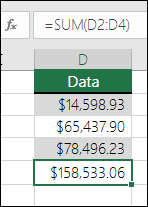
Typos – Imagine trying to enter more and/or much larger values like this:
-
=14598.93+65437.90+78496.23
Then try to validate that your entries are correct. It’s much easier to put these values in individual cells and use a SUM formula. In addition, you can format the values when they’re in cells, making them much more readable then when they’re in a formula.
-
-
#VALUE! errors from referencing text instead of numbers
If you use a formula like:
-
=A1+B1+C1 or =A1+A2+A3
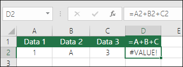
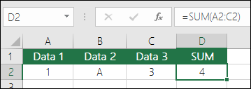
Your formula can break if there are any non-numeric (text) values in the referenced cells, which will return a #VALUE! error. SUM will ignore text values and give you the sum of just the numeric values.
-
-
#REF! error from deleting rows or columns
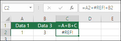
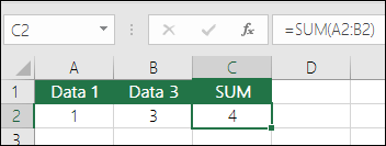
If you delete a row or column, the formula will not update to exclude the deleted row and it will return a #REF! error, where a SUM function will automatically update.
-
Formulas won't update references when inserting rows or columns

If you insert a row or column, the formula will not update to include the added row, where a SUM function will automatically update (as long as you’re not outside of the range referenced in the formula). This is especially important if you expect your formula to update and it doesn’t, as it will leave you with incomplete results that you might not catch.

-
SUM with individual Cell References vs. Ranges
Using a formula like:
-
=SUM(A1,A2,A3,B1,B2,B3)
Is equally error prone when inserting or deleting rows within the referenced range for the same reasons. It’s much better to use individual ranges, like:
-
=SUM(A1:A3,B1:B3)
Which will update when adding or deleting rows.
-
IF Function
The IF function is one of the most popular functions in Excel, and it allows you to make logical comparisons between a value and what you expect.
So an IF statement can have two results. The first result is if your comparison is True, the second if your comparison is False.
For example, =IF(C2=”Yes”,1,2) says IF(C2 = Yes, then return a 1, otherwise return a 2).
Syntax
Use the IF function, one of the logical functions, to return one value if a condition is true and another value if it's false.
IF(logical_test, value_if_true, [value_if_false])
For example:
-
=IF(A2>B2,"Over Budget","OK")
-
=IF(A2=B2,B4-A4,"")
|
Argument name |
Description |
|---|---|
|
logical_test (required) |
The condition you want to test. |
|
value_if_true (required) |
The value that you want returned if the result of logical_test is TRUE. |
|
value_if_false (optional) |
The value that you want returned if the result of logical_test is FALSE. |
Simple IF examples

-
=IF(C2=”Yes”,1,2)
In the above example, cell D2 says: IF(C2 = Yes, then return a 1, otherwise return a 2)

-
=IF(C2=1,”Yes”,”No”)
Common problems
|
Problem |
What went wrong |
|---|---|
|
0 (zero) in cell |
There was no argument for either value_if_true or value_if_False arguments. To see the right value returned, add argument text to the two arguments, or add TRUE or FALSE to the argument. |
|
#NAME? in cell |
This usually means that the formula is misspelled. |


